Matrices

A matrix is an array of numbers arranged with $m$-rows and $n$-columns. When $m=n$ the matrix is termed square. The index of an element in a matrix is notated using the indices $i$ and $j$ for the rows and columns, respectively. For example:

$$\mathbf{B}=
\begin{bmatrix}
b_{11} & b_{12} \\
b_{21} & b_{22} \\
\end{bmatrix}.
$$

The algebra of matrices is straightforward, for example, addition occurs by adding same indexed elements:

$$\mathbf{B}+\mathbf{C} =
\begin{bmatrix}
b_{11}+c_{11} & b_{12}+c_{12} \\
b_{21}+c_{21} & b_{22}+c_{22} \\
\end{bmatrix}
.$$

We can write the addition operation in more compact form using implicit index notation, e.g., $\mathbf{B}+\mathbf{C}=b_{ij}+c_{ij}$. Keep in mind that the dimensions of the matrices must be the same for addition or subtraction operations.

Multiplication of matrices by a scalar quantity is simply, $S\cdot\mathbf{B}$. When multiplying two matrices, the inner dimensions must be the same, for example, if $\mathbf{B}$ is a $m \times n$ then $\mathbf{C}$ must be a $n \times p$. In other words, the number of columns in $\mathbf{B}$ must be equal to the number of rows in $\mathbf{C}$. The operation is written in compact as follows:

$$ c_{jk} = \sum_{i=1}^{n} a_{ji}b_{ik}.$$

Here are some examples, $c_{11} = a_{11}b_{11}+a_{12}b_{21}$ and $c_{12} = a_{11}b_{12} + a_{12}b_{22}$. An important operation/transformation of matrices is the transpose, which is the process of switching elements in the rows and columns. The transpose is indicated with a superscript capital "T", e.g., $\mathbf{B}^T$. For a square matrix, the diagonal components are commonly referred to as the principal terms and the sum of them is the trace of the matrix. For square matrices that have ones as diagonal terms and zeros as off-diagonal terms, we refer to them as unit of identify matrices, for example:

$$\mathbf{I}=\begin{bmatrix}
1 & 0 & 0 \\
0 & 1 & 0 \\
0 & 0 & 1 \\
\end{bmatrix}.$$

Identity matrices are commonly represented with $\mathbf{I}$. Another important property of square matrices is invertibility. A matrix is said to have an inverse if it satisfies the following condition:

$$\mathbf{A}\mathbf{B} = \mathbf{I},$$

we call $\mathbf{B}$ the inverse of $\mathbf{A}$. If a square matrix doesn't have an inverse it is referred to as singular. Matrices that have the inverse which satisfies the condition:

$$\mathbf{A}^{T}\mathbf{A}=\mathbf{I},$$

are orthogonal matrices. A determinant is a specific value that can be computed for square matrices and can be thought of as the scaling factor for linear transformations. The determinant is typically written as:

$$\text{det}\, \mathbf{B} = \Delta \mathbf{B} = |\mathbf{B}|,$$

For 2x2 matrices the determinant is determined by taking the product of the diagonals and subsequent difference between them, as shown below:

$$|\mathbf{B}| =
\begin{vmatrix}
b_{11} & b_{12} \\
b_{21} & b_{22} \\
\end{vmatrix} = b_{11}b_{22}-b_{21}b_{12}.$$

Another method for finding the determinant is using the Laplace expansion method. Determinants have the following commuting properties:

$$|\mathbf{A}\mathbf{B}| = |\mathbf{A}||\mathbf{B}|,$$
$$|\mathbf{A}| = |\mathbf{A}^{T}|.$$

A matrix that is singular will have a determinant that evaluates to zero, thus this is a good way for identifying if a matrix has an inverse.

Matrices and determinants are an important component to the field of  linear algebra, so having good command over them is a serious advantage. I know there are a lot of keywords presented in this post that were not given a formal mathematical description but I strongly suggest clicking the link and reading on to get a better sense of there use in linear algebra.

For this post we will provide a quote from a mathematician who did a lot of research in advance algebra and group theories.

"We [Kaplansky and Halmos] share a philosophy about linear algebra: we think basis-free, we write basis-free, but when the chips are down we close the office door and compute with matrices like fury."
-Irving Kaplansky, Paul Halmos: Celebrating 50 Years of Mathematics

References & Additional Reading

[1] Advanced Engineering Mathematics, Wiley, 8th ed., E. Kreyszig.

[2] The Mathematics Companion, IoP, 1st ed., A.C. Fischer-Cripps.

Reuse and Attribution

Brittle Fracture & Dislocations

Before I dive right into dislocations, let me provide a quick refresher on brittle fracture. From a theoretical perspective, crystalline materials are perfectly repeating spatial structures that lack any defects to disrupt their symmetry. These perfect structures should behave completely elastic, i.e. spring-like, until the onset of fracture due to bond breaking.

Prior to fracture the elastic regime of a crystal's response to loading can be described by anisotropic/isotropic version of Hooke's law : $\sigma_{ij} = C_{ijkl}\epsilon_{kl}$ where $\sigma_{ij}$ is the stress tensor, $\epsilon_{kl}$ is strain tensor, and $C_{ijkl}$ is the stiffness tensor. To describe what happens after the elastic region we require a model for immediate fracture, i.e. fracture occurring at the speed of sound in a material. This event is more commonly referred to as brittle fracture. The most simple model for near perfect brittle fracture is given by the Griffith's criteria. This criteria is based on the stress required to break all the bonds between two atomic planes in order to create a free surface. Typically, the Griffith's criteria is more generally discussed in terms of the stability of a crack with a given length, $l$. For tensile loading, the condition for fracture is given by the equation:

$$ \sigma_{fracture} = \sqrt{\frac{2 E \; \gamma}{\pi \;l}} $$

where $E$ is the Young's modulus , $\gamma$ the surface energy, and $l$ the surface (or crack) length. Therefore, a prototypical brittle material should fracture when $\sigma_{fracture} \leq \sigma_{applied}$. In most cases this is a poor approximation including brittle ceramics, which one might suspect would fit the criteria. The table below provides a few examples of calculated fractured stress for a 0.05 mm crack length of different materials.

Material	$\sigma_{fracture}$[MPa]	E [GPa]	$\gamma$ [mJ/m$^2$]
Silicon	51.6	169	1240
Silica Glass	17.2	75	310
NaCl	12.3	40	300
MgO	61.6	1200	249
CaCO3	15.3	230	80

So why don't metals and engineered materials have brittle fracture characteristics, for example, gold. This is because nature (or man) introduces imperfections into materials that give rise to behavior which deviates from perfect elastic-to-brittle fracture, we call this plasticity meaning non-reversible/permanent deformation.  One major contribution to plasticity are planar defects termed dislocations, these are extra atomic planes that are squeezed in between the parent crystal lattice. In the image below, an example of an edge dislocation is shown.  The dislocation core occurs on the slip plane, i.e., the atomic plan where the dislocation can move about.

Example of a line dislocation with the core marked by the perpendicular symbol. The dashed blue line indicates the slip plane, i.e., the plane for which the dislocation can glide along when a shear force is applied. Once the dislocation reaches a surface it generates a step. Not shown is the burgers vector (adapted from structuredatabase.wordpress.com).

One of the consequences of squeezing extra atomic planes in a host crystal, is the incipient strain/stress fields around dislocations and as a result of this, applying an external load provides enough energy for the dislocation to glide. Dislocations therefore have a mobility associated with them due to these strain/stress fields. This mobility occurs by glide motion along certain atomic planes with a given direction. This magnitude and direction is characterized by the Burgers vector, named after the Dutch physicist, Jan Burgers. For a closed-pack lattice, the magnitude of the Burgers vector along directions $h$,$k$,$l$ (see Miller indices notation post) can be calculated as:

$$ ||\mathbf{b}|| = \frac{a}{2}\sqrt{h^2+k^2+l^2}$$

In association with the Burgers vector is the Burgers circuit, which characterizes the vector magnitude and direction by comparing to a perfect crystal to a dislocation containing crystal.

A complete Burgers circuit for a perfect crystal (left) and the burgers circuit for edge (top-right) and screw (bottom-right) dislocations. As you can see the burgers vector is the extra segment that goes beyond the length of the perfect circuit (adapted from wikipedia)

A perfect example of plasticity induced by dislocations is when a piece of metal is subjected to a shear force. Rather than fracture, as prescribed by Griffith's criteria, dislocations will absorb the applied energy and subsequently move, thereby resulting in plastic or irreversible deformation. In the image shown below produced by Y.-T. Zhou et al. using HRTEM [2], the authors show nicely an edge dislocation in a MnS inclusion inside a steel matrix.

(a) Bright field TEM image of the dislocation distribution in a MnS inclusion. (b) An HRTEM image of the dislocation core. By drawing a closure surrounding the core, the Burgers vector of the dislocation is determined as $\frac{a}{2}[\bar{1}10]$ (figure and caption adapted from ref. [2])

If you would like a more through background on brittle fracture and dislocation dynamics I suggest the text by W.D. Kingery et al. [3] and V. Bulatov and W. Cai [4], respectively. I particularly like the V. Bulatov and W. Cai book since it has excellent exercises to work on. There are also books by Hirth and Lothe and Hull and Bacon focused on introduction to dislocation theory. Now for the selected quote:

“You have to know something to learn something”
-W. David Kingery,  father of modern ceramics, quoted by D. Uhlmann and P. Vandiver

References

[1] The Materials Physics Companion, IoP, 1st ed., A.C. Fischer-Cripps.

[2] Y.-T. Zhou, et al., Philos. Mag. (2015). doi:10.1080/14786435.2015.1052030
[3] Computer Simulations of Dislocations, Oxford Series on Materials Modeling, 1st ed., V. Bulatov and W. Cai
[4] Introduction to Ceramics, Wiley-Interscience, 2nd ed.; W.D. Kingery, H.K. Bowen, D.R. Uhlmann

Reuse and Attribution

Finite Element Method

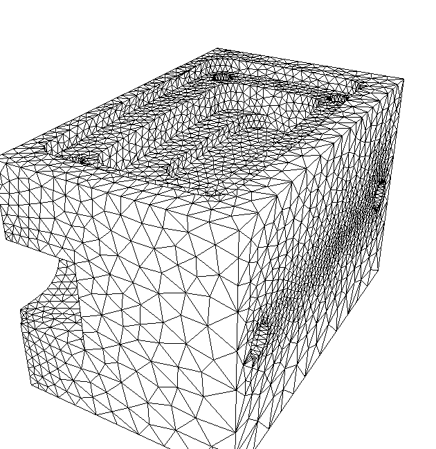
In this blog post, we will consider an elastic response of a solid object under a load $F$ within the framework of finite-element methods (FEM). The purpose of FEM is to discretize the spatial domain of our solid object into several small elements that are connected via nodes. This connectivity is defined by a generated mesh, an example mesh is given in the figure below:

A finite-element 3D triangular mesh example of a part (image adapted from here).

To solve for the displacement or deformation due to an applied load on our solid object, we formulate our problem as a system of equations in terms of matrices, where each matrix represents one element. In our example problem, we make the assumption that the entire structure is in equilibrium and thus each element must also be in equilibrium. To find the displacement at each node we use Hooke's law for elastic response:

$$ \mathbf{\sigma} = \mathbf{E}\cdot\mathbf{\epsilon}$$

where $\mathbf{\sigma}$ is the stress, $E$ Young's modulus, and $\epsilon$ the strain. The strain is given by the following displacement node matrix,

\[\mathbf{\epsilon}=\begin{bmatrix}\frac{\partial}{\partial x} & 0 \\ 0 & \frac{\partial}{\partial y} \\ \frac{\partial}{\partial y} & \frac{\partial}{\partial x} \end{bmatrix}\mathbf{u}\]

here $\mathbf{u}$ is the node displacement. In matrix notation, Hooke's law reads,

\[\mathbf{\sigma} = \frac{E}{\left(1+\nu\right)\left(1+2\nu\right)}\begin{bmatrix}1-\nu & & \\ \nu & 1-\nu & \\ & & \frac{\left(1-2\nu\right)}{2}\end{bmatrix}\mathbf{\epsilon}\]

As mentioned the solid body is in mechanical equilibrium and so the work being done by external loads balances with the work done by internal forces. The equilibrium of node $i$ acted on by force, $F_i$, is written as:

$$\delta \mathbf{u}_{i}^T\mathbf{F}_i = \int_{V} \delta \mathbf{\epsilon}^{T}\mathbf{\sigma}dV$$

The integrand can then be expressed in terms of the element stiffness matrix, $\mathbf{K}$, and displacements at node $i$ can be solved for the applied load. The operations would be:

1. Assemble the stiffness matrix $\mathbf{K}$
2. Apply boundary conditions
3. Calculate the displacements at each node $i$ by solving the equation:  

       $$ \mathbf{u}_i = \mathbf{K}^{-1}\mathbf{P}_i$$

where $\mathbf{P}_i$ is the applied load at each node. The majority of the effort in FEM is the inversion of the stiffness matrix. Due to the complexity of the mesh and geometry, numerical methods are typically used to solve FEM problems.

I hope this was a useful refresher to FEM, if you have any suggestions feel free to add them in the comment section. Finding a quote for this post was no easy task but I found this one which I slightly modified:

"The innards of Ping's G5 golf club were supposedly computer-engineered with a process called finite-element analysis, a term that for all I know was stolen from a Star Trek episode."
-Carl Hiaasen, The Downhill Lie: A Hacker's Return to a Ruinous Sport 

References  & Additional Reading

[1] Advanced Engineering Mathematics, Wiley, 8th ed., E. Kreyszig.

[2] The Mathematics Companion, IoP, 1st ed., A.C. Fischer-Cripps.

Reuse and Attribution